Double 2D Sersic example

In this example we create a (simplified) synthetic galaxy image consisting of two Sersic components, add some “realism” to it (PSF + noise), and then run statmorph in order to recover the parameters of the two components.

import numpy as np
import matplotlib.pyplot as plt
from astropy.visualization import simple_norm
from astropy.modeling.models import Sersic2D
from astropy.convolution import convolve, Gaussian2DKernel
from photutils.segmentation import detect_threshold, detect_sources
import time
import statmorph
%matplotlib inline

Setting up

Creating the model galaxy image

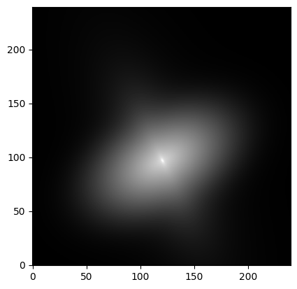
We assume that the image size is 240x240 pixels and that the “true” light distribution corresponds to a double 2D Sersic model with the following parameters (note that the two components share the same center, by construction):

ny, nx = 240, 240
y, x = np.mgrid[0:ny, 0:nx]
doublesersic_model = statmorph.DoubleSersic2D(
    x_0=120.5, y_0=96.5,
    amplitude_1=1, r_eff_1=10, n_1=5.0, ellip_1=0.6, theta_1=2.0,
    amplitude_2=2, r_eff_2=20, n_2=1.0, ellip_2=0.4, theta_2=0.5)
image = doublesersic_model(x, y)

# Visualize "idealized" image
plt.imshow(image, cmap='gray', origin='lower',
           norm=simple_norm(image, stretch='log', log_a=10000))

<matplotlib.image.AxesImage at 0x7f2c2fbb0f10>

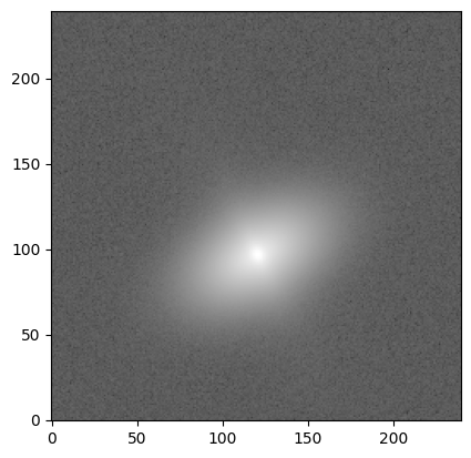
Applying realism

We now apply some “realism” (PSF + noise) to the idealized image (see the tutorial for more details):

# Convolve with PSF
kernel = Gaussian2DKernel(2.0)
kernel.normalize()  # make sure kernel adds up to 1
psf = kernel.array  # we only need the numpy array
image = convolve(image, psf)

# Apply shot noise
np.random.seed(3)
gain = 1e5
image = np.random.poisson(image * gain) / gain

# Apply background noise
sky_sigma = 0.01
image += sky_sigma * np.random.standard_normal(size=(ny, nx))

# Visualize "realistic" image
plt.imshow(image, cmap='gray', origin='lower',
           norm=simple_norm(image, stretch='log', log_a=10000))

<matplotlib.image.AxesImage at 0x7f2c27ff5a10>

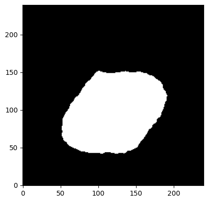
Creating a segmentation map

We also need to create a segmentation image (see the tutorial for more details):

threshold = detect_threshold(image, 1.5)
npixels = 5  # minimum number of connected pixels
convolved_image = convolve(image, psf)
segmap = detect_sources(convolved_image, threshold, npixels)
plt.imshow(segmap, origin='lower', cmap='gray')

<matplotlib.image.AxesImage at 0x7f2c27fd36d0>

Running statmorph

We now have all the input necessary to run statmorph. However, unlike in the tutorial, this time we include the option include_doublesersic = True, which is necessary in order to carry out the double Sersic fit.

start = time.time()
source_morphs = statmorph.source_morphology(
    image, segmap, gain=gain, psf=psf, include_doublesersic=True)
print('Time: %g s.' % (time.time() - start))

Time: 5.49718 s.

Examining the output

We focus on the first (and only) source labeled in the segmap:

morph = source_morphs[0]

We print some of the morphological properties just calculated:

print('BASIC MEASUREMENTS (NON-PARAMETRIC)')
print('xc_centroid =', morph.xc_centroid)
print('yc_centroid =', morph.yc_centroid)
print('ellipticity_centroid =', morph.ellipticity_centroid)
print('elongation_centroid =', morph.elongation_centroid)
print('orientation_centroid =', morph.orientation_centroid)
print('xc_asymmetry =', morph.xc_asymmetry)
print('yc_asymmetry =', morph.yc_asymmetry)
print('ellipticity_asymmetry =', morph.ellipticity_asymmetry)
print('elongation_asymmetry =', morph.elongation_asymmetry)
print('orientation_asymmetry =', morph.orientation_asymmetry)
print('rpetro_circ =', morph.rpetro_circ)
print('rpetro_ellip =', morph.rpetro_ellip)
print('rhalf_circ =', morph.rhalf_circ)
print('rhalf_ellip =', morph.rhalf_ellip)
print('r20 =', morph.r20)
print('r80 =', morph.r80)
print('Gini =', morph.gini)
print('M20 =', morph.m20)
print('F(G, M20) =', morph.gini_m20_bulge)
print('S(G, M20) =', morph.gini_m20_merger)
print('sn_per_pixel =', morph.sn_per_pixel)
print('C =', morph.concentration)
print('A =', morph.asymmetry)
print('S =', morph.smoothness)
print()
print('SINGLE SERSIC')
print('sersic_amplitude =', morph.sersic_amplitude)
print('sersic_rhalf =', morph.sersic_rhalf)
print('sersic_n =', morph.sersic_n)
print('sersic_xc =', morph.sersic_xc)
print('sersic_yc =', morph.sersic_yc)
print('sersic_ellip =', morph.sersic_ellip)
print('sersic_theta =', morph.sersic_theta)
print('sersic_chi2_dof =', morph.sersic_chi2_dof)
print('sersic_aic =', morph.sersic_aic)
print('sersic_bic =', morph.sersic_bic)
print()
print('DOUBLE SERSIC')
print('doublesersic_xc =', morph.doublesersic_xc)
print('doublesersic_yc =', morph.doublesersic_yc)
print('doublesersic_amplitude1 =', morph.doublesersic_amplitude1)
print('doublesersic_rhalf1 =', morph.doublesersic_rhalf1)
print('doublesersic_n1 =', morph.doublesersic_n1)
print('doublesersic_ellip1 =', morph.doublesersic_ellip1)
print('doublesersic_theta1 =', morph.doublesersic_theta1)
print('doublesersic_amplitude2 =', morph.doublesersic_amplitude2)
print('doublesersic_rhalf2 =', morph.doublesersic_rhalf2)
print('doublesersic_n2 =', morph.doublesersic_n2)
print('doublesersic_ellip2 =', morph.doublesersic_ellip2)
print('doublesersic_theta2 =', morph.doublesersic_theta2)
print('doublesersic_chi2_dof =', morph.doublesersic_chi2_dof)
print('doublesersic_aic =', morph.doublesersic_aic)
print('doublesersic_bic =', morph.doublesersic_bic)
print()
print('OTHER')
print('sky_mean =', morph.sky_mean)
print('sky_median =', morph.sky_median)
print('sky_sigma =', morph.sky_sigma)
print('flag =', morph.flag)
print('flag_sersic =', morph.flag_sersic)
print('flag_doublesersic =', morph.flag_doublesersic)

BASIC MEASUREMENTS (NON-PARAMETRIC)
xc_centroid = 120.49796915600066
yc_centroid = 96.49072665561145
ellipticity_centroid = 0.3281195014248586
elongation_centroid = 1.4883599123961813
orientation_centroid = 0.5084303360046819
xc_asymmetry = 120.50349931366914
yc_asymmetry = 96.49787567701722
ellipticity_asymmetry = 0.3281195422315757
elongation_asymmetry = 1.4883600027918478
orientation_asymmetry = 0.5084304950285234
rpetro_circ = 33.36098569267929
rpetro_ellip = 39.842823133428446
rhalf_circ = 15.096079572335228
rhalf_ellip = 18.21255967425545
r20 = 6.539984509831923
r80 = 26.432815995577958
Gini = 0.5074708179797278
M20 = -1.9551333404024447
F(G, M20) = -0.09311204610145296
S(G, M20) = -0.09636742451600933
sn_per_pixel = 144.75915247089574
C = 3.032833565360866
A = 0.0010288533244274547
S = 0.010715553260193519

SINGLE SERSIC
sersic_amplitude = 1.967639259495446
sersic_rhalf = 18.530416288731864
sersic_n = 1.5844860752707133
sersic_xc = 120.50045625459862
sersic_yc = 96.49964597762032
sersic_ellip = 0.2878868948405022
sersic_theta = 0.5187753221125859
sersic_chi2_dof = 22.69106134737694
sersic_aic = 179826.2894772886
sersic_bic = 179889.01817915562

DOUBLE SERSIC
doublesersic_xc = 120.50104504377103
doublesersic_yc = 96.49987575162125
doublesersic_amplitude1 = 0.9979493447212455
doublesersic_rhalf1 = 10.009773788312145
doublesersic_n1 = 4.987096758590505
doublesersic_ellip1 = 0.5987696184404921
doublesersic_theta1 = 2.0007785239089033
doublesersic_amplitude2 = 1.9994925627936888
doublesersic_rhalf2 = 20.00028009044196
doublesersic_n2 = 0.9995604986519387
doublesersic_ellip2 = 0.4001378286835756
doublesersic_theta2 = 0.5001989199379825
doublesersic_chi2_dof = 0.9512591117625556
doublesersic_aic = -2866.1036815325647
doublesersic_bic = -2758.5687640462575

OTHER
sky_mean = 0.0009549396027924723
sky_median = 0.0006752941207164413
sky_sigma = 0.01025075780746779
flag = 0
flag_sersic = 0
flag_doublesersic = 0

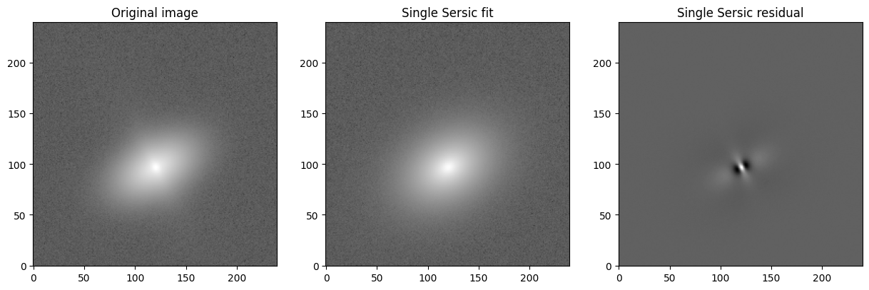
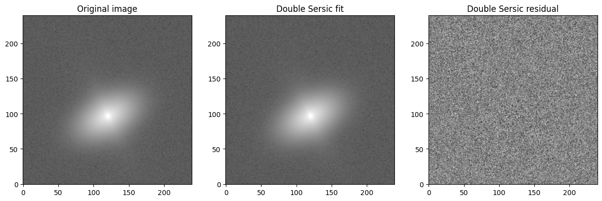
Clearly, the fitted double Sersic model is consistent with the “true” light distribution that we originally created (n1 = 5, n2 = 1, etc.) and the reduced chi-squared statistic (doublesersic_chi2_dof) is close to 1, indicating a good fit without overfitting. On the other hand, the single Sersic fit has a reduced chi-squared statistic much larger than 1, indicating a poor fit (as expected).

We also calculate the Akaike Information Criterion (AIC) and Bayesian Information Criterion (BIC) for the two models, which again favor the double Sersic model as the statistically preferred one, since it returns much lower AIC and BIC values.

Also note that statmorph now returns an additional quality flag:

• flag_doublesersic : indicates the quality of the double Sersic fit. Like flag and flag_sersic, it can take the following values: 0 (good), 1 (suspect), 2 (bad), and 4 (catastrophic).

Visualizing the individual components

For some applications (e.g. bulge/disk decompositions) it might be useful to analyze the two fitted components separately, as we do below.

ny, nx = image.shape
y, x = np.mgrid[0:ny, 0:nx]
sersic1 = Sersic2D(morph.doublesersic_amplitude1,
                   morph.doublesersic_rhalf1,
                   morph.doublesersic_n1,
                   morph.doublesersic_xc,
                   morph.doublesersic_yc,
                   morph.doublesersic_ellip1,
                   morph.doublesersic_theta1)
sersic2 = Sersic2D(morph.doublesersic_amplitude2,
                   morph.doublesersic_rhalf2,
                   morph.doublesersic_n2,
                   morph.doublesersic_xc,
                   morph.doublesersic_yc,
                   morph.doublesersic_ellip2,
                   morph.doublesersic_theta2)
image1 = sersic1(x, y)
image2 = sersic2(x, y)
image_total = image1 + image2

fig = plt.figure(figsize=(15,5))
ax = fig.add_subplot(131)
ax.imshow(image1, cmap='gray', origin='lower',
           norm=simple_norm(image_total, stretch='log', log_a=10000))
ax.set_title('First component')
ax.text(0.04, 0.93, 'n1 = %.4f' % (morph.doublesersic_n1,),
        bbox=dict(facecolor='white'), transform=ax.transAxes)
ax = fig.add_subplot(132)
ax.imshow(image2, cmap='gray', origin='lower',
           norm=simple_norm(image_total, stretch='log', log_a=10000))
ax.set_title('Second component')
ax.text(0.04, 0.93, 'n2 = %.4f' % (morph.doublesersic_n2,),
        bbox=dict(facecolor='white'), transform=ax.transAxes)
ax = fig.add_subplot(133)
ax.imshow(image_total, cmap='gray', origin='lower',
           norm=simple_norm(image_total, stretch='log', log_a=10000))
ax.set_title('Composite model')

Text(0.5, 1.0, 'Composite model')

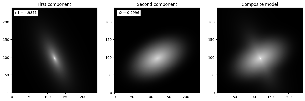
Note that the two Sersic components shown above are not convolved with the PSF, since they are meant to recover the “true” light distributions of the two components of the galaxy.

Examining the single Sersic fit

For illustration puposes, below we compare the original (realistic) image to the single Sersic fit.

bg_noise = sky_sigma * np.random.standard_normal(size=(ny, nx))
model = statmorph.ConvolvedSersic2D(
    morph.sersic_amplitude,
    morph.sersic_rhalf,
    morph.sersic_n,
    morph.sersic_xc,
    morph.sersic_yc,
    morph.sersic_ellip,
    morph.sersic_theta)
model.set_psf(psf)  # must set PSF by hand
image_model = model(x, y)

fig = plt.figure(figsize=(15,5))
ax = fig.add_subplot(131)
ax.imshow(image, cmap='gray', origin='lower',
           norm=simple_norm(image, stretch='log', log_a=10000))
ax.set_title('Original image')
ax = fig.add_subplot(132)
ax.imshow(image_model + bg_noise, cmap='gray', origin='lower',
           norm=simple_norm(image, stretch='log', log_a=10000))
ax.set_title('Single Sersic fit')
ax = fig.add_subplot(133)
residual = image - image_model
ax.imshow(residual, cmap='gray', origin='lower',
           norm=simple_norm(residual, stretch='linear'))
ax.set_title('Single Sersic residual')

Text(0.5, 1.0, 'Single Sersic residual')

Examining the double Sersic fit

Similarly, below we compare the original (realistic) image to the double Sersic fit.

model = statmorph.ConvolvedDoubleSersic2D(
    morph.doublesersic_xc,
    morph.doublesersic_yc,
    morph.doublesersic_amplitude1,
    morph.doublesersic_rhalf1,
    morph.doublesersic_n1,
    morph.doublesersic_ellip1,
    morph.doublesersic_theta1,
    morph.doublesersic_amplitude2,
    morph.doublesersic_rhalf2,
    morph.doublesersic_n2,
    morph.doublesersic_ellip2,
    morph.doublesersic_theta2)
model.set_psf(psf)  # must set PSF by hand
image_model = model(x, y)

fig = plt.figure(figsize=(15,5))
ax = fig.add_subplot(131)
ax.imshow(image, cmap='gray', origin='lower',
           norm=simple_norm(image, stretch='log', log_a=10000))
ax.set_title('Original image')
ax = fig.add_subplot(132)
ax.imshow(image_model + bg_noise, cmap='gray', origin='lower',
           norm=simple_norm(image, stretch='log', log_a=10000))
ax.set_title('Double Sersic fit')
ax = fig.add_subplot(133)
residual = image - image_model
ax.imshow(residual, cmap='gray', origin='lower',
           norm=simple_norm(residual, stretch='linear'))
ax.set_title('Double Sersic residual')

Text(0.5, 1.0, 'Double Sersic residual')

fig.savefig('doublesersic.png', dpi=150)
plt.close(fig)

Concluding remarks

The fact that statmorph uses Astropy’s modeling utility behind the scenes provides a great deal of flexibility. For example, if one is interested in fitting a de Vaucouleurs + exponential model (these components are, of course, special cases of the Sersic model with n = 4 and n = 1, respectively), one simply has to add the following option when calling statmorph:

doublesersic_model_args = {
    'n_1': 4, 'n_2': 1, 'fixed': {'n_1': True, 'n_2': True}}

Furthermore, in some applications it might make sense to “tie” the ellipticity and position angle of the two Sersic components. This can also be accomplished using doublesersic_model_args in combination with the tied property of Astropy parameters, although the syntax is slightly more involved (more details here). Alternatively, statmorph provides the following option for this purpose, which achieves the same effect:

doublesersic_tied_ellip = True