Tutorial / How to use

In this tutorial we create a (simplified) synthetic galaxy image from scratch, along with its associated segmentation map, and then run the statmorph code on it.

If you already have a real astronomical image and segmentation map to work with, jump to Running statmorph.

Setting up

We import some Python packages first. If you are missing any of these, please see the the installation instructions.

import numpy as np
import matplotlib.pyplot as plt
from astropy.visualization import simple_norm
from astropy.modeling.models import Sersic2D
from astropy.convolution import convolve, Gaussian2DKernel
from photutils.segmentation import detect_threshold, detect_sources
import time
import statmorph
%matplotlib inline

Creating a model galaxy image

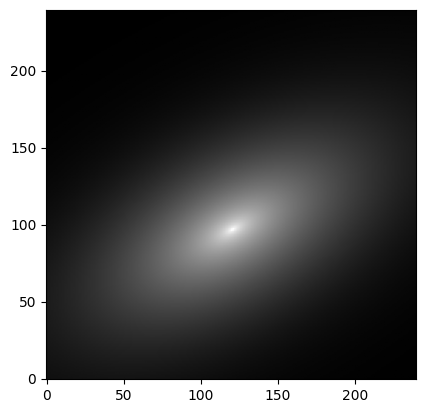
We assume that the image size is 240x240 pixels and that the “true” light distribution is described by a 2D Sersic model with the following parameters:

ny, nx = 240, 240
y, x = np.mgrid[0:ny, 0:nx]
sersic_model = Sersic2D(
    amplitude=1, r_eff=20, n=2.5, x_0=120.5, y_0=96.5,
    ellip=0.5, theta=0.5)
image = sersic_model(x, y)
plt.imshow(image, cmap='gray', origin='lower',
           norm=simple_norm(image, stretch='log', log_a=10000))

<matplotlib.image.AxesImage at 0x7f9c3622a650>

Convolving with a PSF

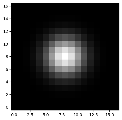
In practice, every astronomical image is the convolution of a “true” image with a point spread function (PSF), which depends on the optics of the telescope, atmospheric conditions, etc. Here we assume that the PSF is a simple 2D Gaussian kernel with a standard deviation of 2 pixels:

kernel = Gaussian2DKernel(2)
kernel.normalize()  # make sure kernel adds up to 1
psf = kernel.array  # we only need the numpy array
plt.imshow(psf, origin='lower', cmap='gray')

<matplotlib.image.AxesImage at 0x7f9c362f6e10>

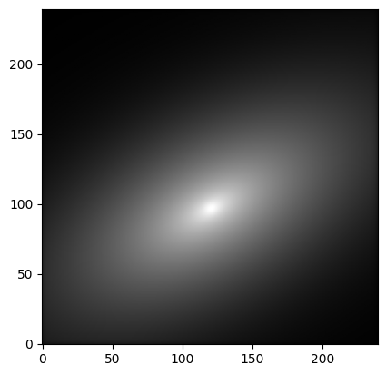
Now we convolve the image with the PSF.

image = convolve(image, psf)
plt.imshow(image, cmap='gray', origin='lower',
           norm=simple_norm(image, stretch='log', log_a=10000))

<matplotlib.image.AxesImage at 0x7f9c340f29d0>

Applying shot noise

One source of noise in astronomical images originates from the Poisson statistics of the number of electrons recorded by each pixel. We can model this effect by introducing a gain parameter, a scalar that can be multiplied by the science image to obtain the number of electrons per pixel.

For the sake of this example, we choose a very large gain value, so that shot noise becomes almost negligible (10^5 electrons/pixel at the effective radius, where we had defined an amplitude of 1.0 in arbitrary units). The resulting image after applying shot noise looks very similar to the one from the previous step and is not shown.

np.random.seed(3)
gain = 1e5
image = np.random.poisson(image * gain) / gain

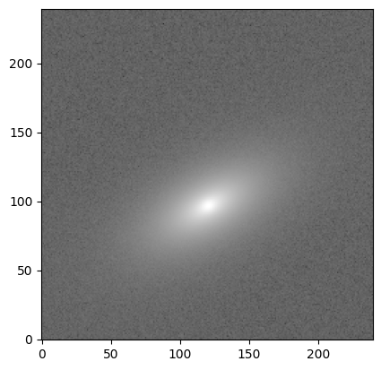
Applying background noise

Apart from shot noise, astronomical images have a sky background noise component, which we here model with a uniform Gaussian distribution centered at zero (since the image is background-subtracted).

We assume, somewhat optimistically, that the signal-to-noise ratio (S/N) per pixel is 100 at the effective radius (where we had defined the Sersic model amplitude as 1.0).

snp = 100.0
sky_sigma = 1.0 / snp
image += sky_sigma * np.random.standard_normal(size=(ny, nx))
plt.imshow(image, cmap='gray', origin='lower',
           norm=simple_norm(image, stretch='log', log_a=10000))

<matplotlib.image.AxesImage at 0x7f9c340eb850>

Gain and weight maps

Note that statmorph will ask for one of two input arguments: (1) a weight map, which is a 2D array (of the same size as the input image) representing one standard deviation at each pixel value, or (2) the gain, which was described above. In the latter case, the gain parameter is used internally by statmorph (along with an automatic estimation of the sky background noise) to calculate the weight map.

Creating a segmentation map

Besides the image itself and the weight map/gain, the only other required argument is the segmentation map, which labels the pixels belonging to different sources. It is usually generated with specialized tools such as SExtractor or photutils. Here we use the latter to create a simplified segmentation map, where we detect sources that lie above a 1.5-sigma detection threshold.

Note that the detection stage (but, importantly, not the threshold calculation) is carried out on a “convolved” version of the image. This is done in order to smooth out small-scale noise and thus ensure that the shapes of the detected segments are reasonably smooth.

threshold = detect_threshold(image, 1.5)
npixels = 5  # minimum number of connected pixels
convolved_image = convolve(image, psf)
segmap = detect_sources(convolved_image, threshold, npixels)
plt.imshow(segmap, origin='lower', cmap='gray')

<matplotlib.image.AxesImage at 0x7f9c3412f750>

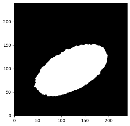
In this particular case, the obtained segmap has only two values: 0 for the background (as should always be the case) and 1 for the only labeled source. However, statmorph is designed to process all the sources labeled by a segmentation map, which makes it applicable to large mosaic images.

Running statmorph

Now that we have all the required data, we are ready to measure the morphology of the source just created. Note that we include the PSF as a keyword argument, which results in more correct Sersic profile fits.

Also note that we do not attempt to fit a double Sersic model, which would be degenerate in this particular case (the two components would be identical and their relative amplitudes would be unconstrained). For a demonstration of statmorph’s double Sersic fitting functionality, see the Double 2D Sersic example.

start = time.time()
source_morphs = statmorph.source_morphology(
    image, segmap, gain=gain, psf=psf)
print('Time: %g s.' % (time.time() - start))

Time: 1.63648 s.

Examining the output

In general, source_morphs is a list of objects corresponding to each labeled source in the image. Here we focus on the first (and only) labeled source:

morph = source_morphs[0]

Now we print some of the morphological properties just calculated:

print('BASIC MEASUREMENTS (NON-PARAMETRIC)')
print('xc_centroid =', morph.xc_centroid)
print('yc_centroid =', morph.yc_centroid)
print('ellipticity_centroid =', morph.ellipticity_centroid)
print('elongation_centroid =', morph.elongation_centroid)
print('orientation_centroid =', morph.orientation_centroid)
print('xc_asymmetry =', morph.xc_asymmetry)
print('yc_asymmetry =', morph.yc_asymmetry)
print('ellipticity_asymmetry =', morph.ellipticity_asymmetry)
print('elongation_asymmetry =', morph.elongation_asymmetry)
print('orientation_asymmetry =', morph.orientation_asymmetry)
print('rpetro_circ =', morph.rpetro_circ)
print('rpetro_ellip =', morph.rpetro_ellip)
print('rhalf_circ =', morph.rhalf_circ)
print('rhalf_ellip =', morph.rhalf_ellip)
print('r20 =', morph.r20)
print('r80 =', morph.r80)
print('Gini =', morph.gini)
print('M20 =', morph.m20)
print('F(G, M20) =', morph.gini_m20_bulge)
print('S(G, M20) =', morph.gini_m20_merger)
print('sn_per_pixel =', morph.sn_per_pixel)
print('C =', morph.concentration)
print('A =', morph.asymmetry)
print('S =', morph.smoothness)
print()
print('SERSIC MODEL')
print('sersic_amplitude =', morph.sersic_amplitude)
print('sersic_rhalf =', morph.sersic_rhalf)
print('sersic_n =', morph.sersic_n)
print('sersic_xc =', morph.sersic_xc)
print('sersic_yc =', morph.sersic_yc)
print('sersic_ellip =', morph.sersic_ellip)
print('sersic_theta =', morph.sersic_theta)
print('sersic_chi2_dof =', morph.sersic_chi2_dof)
print()
print('OTHER')
print('sky_mean =', morph.sky_mean)
print('sky_median =', morph.sky_median)
print('sky_sigma =', morph.sky_sigma)
print('flag =', morph.flag)
print('flag_sersic =', morph.flag_sersic)

BASIC MEASUREMENTS (NON-PARAMETRIC)
xc_centroid = 120.52691025551975
yc_centroid = 96.50830357120901
ellipticity_centroid = 0.4916290565698266
elongation_centroid = 1.9670675771762582
orientation_centroid = 0.49924368928600915
xc_asymmetry = 120.49527157443472
yc_asymmetry = 96.49566691576838
ellipticity_asymmetry = 0.4916296269595144
elongation_asymmetry = 1.9670697842188416
orientation_asymmetry = 0.4992433053842231
rpetro_circ = 32.11308037499967
rpetro_ellip = 43.330238512205305
rhalf_circ = 14.64102614422408
rhalf_ellip = 19.17778559718613
r20 = 5.07248910571569
r80 = 26.138890433454648
Gini = 0.5687616162705555
M20 = -2.078304915699426
F(G, M20) = 0.29563530711895236
S(G, M20) = -0.05281038317437026
sn_per_pixel = 81.19953322323099
C = 3.560330126795657
A = -0.001320789204492828
S = 0.007699689253035814

SERSIC MODEL
sersic_amplitude = 1.0002097553046503
sersic_rhalf = 19.995363146001612
sersic_n = 2.5001097998051005
sersic_xc = 120.50019215407934
sersic_yc = 96.49895458342795
sersic_ellip = 0.4999262253919466
sersic_theta = 0.5001726455732174
sersic_chi2_dof = 0.937596910478335

OTHER
sky_mean = 0.004674857464116049
sky_median = 0.004651799083317322
sky_sigma = 0.010258725331952904
flag = 0
flag_sersic = 0

Note that the fitted Sersic model is in very good agreement with the “true” Sersic model that we originally defined (n = 2.5, rhalf = 20, etc.) and that the reduced chi-squared statistic (sersic_chi2_dof) is close to 1, indicating a good fit without overfitting. However, such good agreement tends to deteriorate somewhat at higher noise levels, and one has to keep in mind that not all galaxies are well described by Sersic profiles.

Other morphological measurements that are more general and robust to noise, which are also calculated by statmorph, include the Gini-M20 (Lotz et al. 2004), CAS (Conselice 2003) and MID (Freeman et al. 2013) statistics, as well as the RMS asymmetry (Sazonova et al. 2024), outer asymmetry (Wen et al. 2014), and shape asymmetry (Pawlik et al. 2016).

Also note that statmorph returns two quality flags:

1. flag : indicates the quality of the basic morphological measurements, taking one of the following values: 0 (good), 1 (suspect), 2 (bad), or 4 (catastrophic). More details can be found here.

2. flag_sersic : indicates the quality of the Sersic fit, also taking values of 0 (good), 1 (suspect), 2 (bad), or 4 (catastrophic).

In general, flag <= 1 should always be enforced, while flag_sersic <= 1 should only be used when one is interested in the Sersic fits (which might fail for merging galaxies and other “irregular” objects).

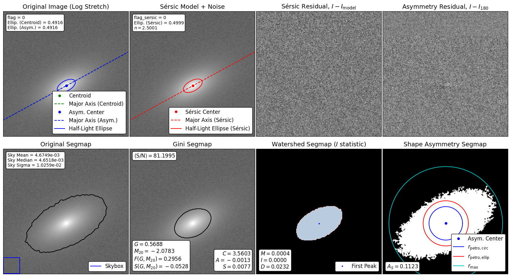
Visualizing the morphological measurements

For convenience, statmorph includes a make_figure function that can be used to visualize some of the morphological measurements. This creates a multi-panel figure analogous to Fig. 4 from Rodriguez-Gomez et al. (2019).

from statmorph.utils.image_diagnostics import make_figure
fig = make_figure(morph)

fig.savefig('tutorial.png', dpi=150)
plt.close(fig)